Beginner’s Guide to Pivoting Data Frames in R

A step by step tutorial on how to convert a wide data frame to a long one

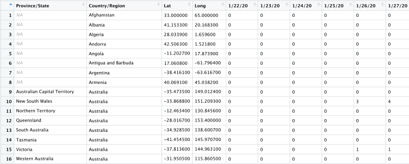
Many-a-times data collection happens in a column-by-column fashion. That means for every new data series we create a new column in our data table. E.g. John Hopkins COVID-19 dataset is built like that. A new column is added for every new day.

This results in very wide data frames. Such wide data frames are generally difficult to analyse. R language’s tidyverse library provides us with a very neat method to pivot our data frame from a wide format to a long one. Let’s take a look at a few examples.

Basic Pivot Longer

pivot_longer() makes datasets longer by increasing the number of rows and decreasing the number of columns. To illustrate the most basic use of pivot_longer function we generate a dummy dataset using tribble() method.

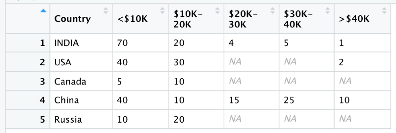
Income Data Country-wise

This dummy dataset contains a country’s wealth distribution. Each row corresponds to a single country. It contains country’s name, and the percentage of people in one of the five wealth categories.

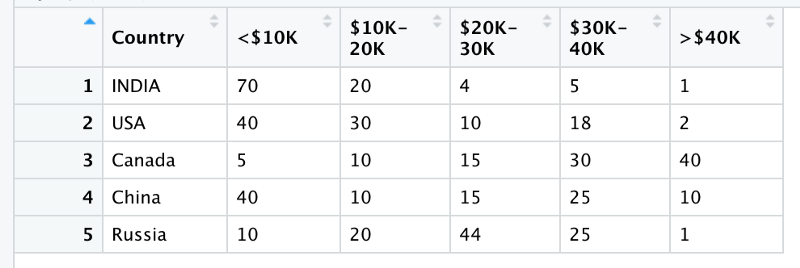
Now this is a wide format let’s convert it into a long format. In the long format we will have only 3 columns

1. Country name
2. Income category
3. Percentage of people in that category

income_data <- dummy_data_1 %>%
  pivot_longer(-c(Country), names_to = "income", values_to = "percentage")

Points to be noted

• dummy_data_1 is the input data (created by using tribble method)
• income_data is the output data frame
• %>% is the pipe operator. Basically, anything that comes after the pipe is applied to anything that comes before it. This article explains how piping works in R
• pivot_longer is applied to dummy_data_1
• -c(Country) tells pivot_longer to pivot everything except Country (minus sign means except)
• names_to gives the name of the variable that will be created from the data stored in the column names, i.e. income.
• values_to gives the name of the variable that will be created from the data stored in the cell value, i.e. percentage.

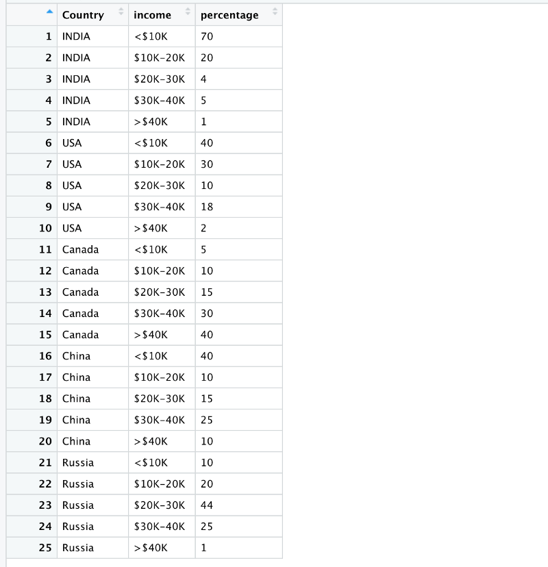
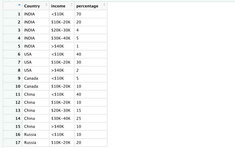
Let’s look at how the final income_data looks like

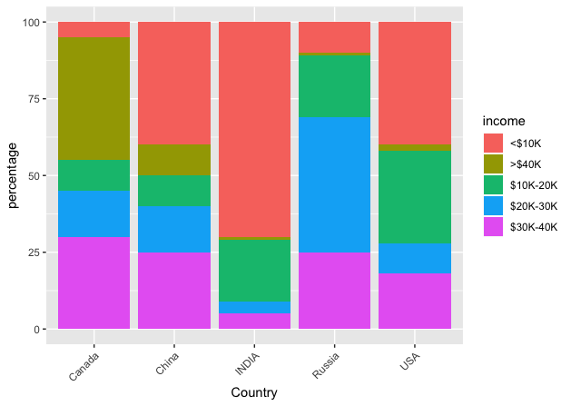
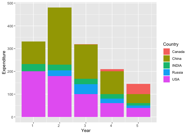
It then becomes extremely easy to plot this data.

Handling Missing Values in Pivot Longer

What if some of the cells have NA values. After pivoting these cells will become rows with no information. It is best to remove these rows during the pivot itself.

Remove NA after pivoting

income_data_drop <- dummy_data %>%
  pivot_longer(-c(Country), names_to = "income", values_to = "percentage", values_drop_na = TRUE)

Note the values_drop_na field. It is used inside pivot_longer function and automatically drops any rows from the final data frame that have percentage=NA.

From 25 rows we are down to 17 now.

Numerical Data in Column Names

Sometimes column names in a wide data frame have numerical information in them. For example, day numbers or week numbers, or school id etc. We might want to extract out this numerical information while pivoting and inject it into our long data frame.

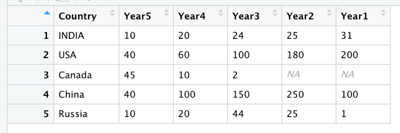
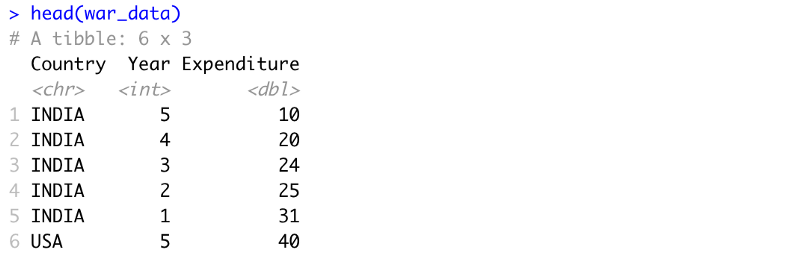
Let’s take another dummy dataset. This Dummy Dataset contains a country’s expenditure on wars in the last 5 years. Each row contains country’s name, and amount of dollars spent in war in 5 years. Year5 means 5 years in the past.

Let’s pivot it.

war_data <- dummy_data_2 %>%
  pivot_longer(
    cols = starts_with("Year"), 
    names_to = "Year", 
    values_to = "Expenditure", 
    values_drop_na = TRUE
  )

Earlier we mentioned which columns to not pivot. Now we have mentioned which columns to include in pivoting. After pivoting the top 6rows of the war_data look like this

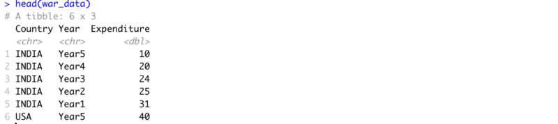
We are left with 3 columns only. But we can clearly see that the year column should be a numerical column. Right now it is a character string.

Changing type of a column

We can change the type of a column by adding 2 more fields to our pivot_longer.

• names_prefix strips off the Year prefix, and
• names_ptypes specifies that Year should be an integer:

war_data <- dummy_data_2 %>%
  pivot_longer(
    cols = starts_with("Year"), 
    names_to = "Year", 
    names_prefix = "Year",
    names_ptypes = list(Year = integer()),
    values_to = "Expenditure",
    values_drop_na = TRUE
  )

The year column is now an integer.

Multiple Variables

Till now a row contained data corresponding to a single variable like expenditure, or percentage population. What if each row has more than 1 variable. For example, in the previous example we have yearly expenditure data for each country, but what if we had another variable apart from expenditure! How would we differentiate them?

Let’s consider an Olympics example. This 3rd dummy dataset contains a country’s olympic medal count across the years in different sports by the 2 genders. Each row contains country-name, and the number of different gold, silver and bronze medals in swimming and hockey by male and female players over the last 50 years. This means 3 variables.

Variables — Medal Type, Sport Type and Gender of The Sportsperson.

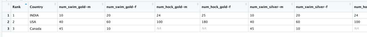
There are 3 types of columns

• Column 1 — Rank
• Column 2 — Country Name
• Column 3:14 — Number of medals

The names of the 3rd type are of the following form

num_<sport>_<medal_type>-<gender>
e.g.
num_swim_gold-f (Number of gold medals in Female Swimming Category)

Now ideally all these variables should form their own column. We cannot use the pivot_longer as it is. Let’s see how to pivot it.

medal_data <- dummy_data_3 %>%
  pivot_longer(
    cols = -c(Rank, Country), 
    names_to = c("Sport", "Medal", "Gender"), 
    names_pattern = "num_(.*)_(.*)-(.)",
    values_to = "Count",
    values_drop_na = TRUE
  )

Points to be noted

• names_to now has more than 1 field.
• names_to has 3 fields which means we will have to identify these 3 variables in column names
• names_pattern contains the regular expression we will need to extract values for the 3 fields stated in names_to

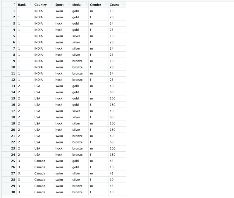
The regular expression “num_(.*)_(.*)-(.)” works as follows

• It ignores the string num and matches anything between the next 2 underscores
• The matched string is passed to the column Sport
• Then it tries to match anything between an underscore and a dash.
• The matched string is passed to the column Medal
• Then it tries to match alphabet after the dash.
• The matched string is passed to the Gender column

Duplicate Column Names

Very rarely bad architecture design leads to repeated column names. Ideally this shouldn’t occur but R has provisions to pivot even these kinds of wide data frames.

Let’s take a look at our last dummy dataset. This contains house ownership data. Each row contains the name of the owner and three cities where she has a house.

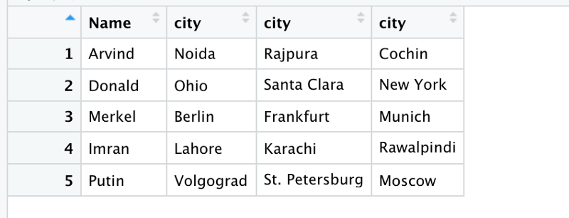
One doesn’t need to do anything special to pivot it.

housing_data <- dummy_data_5 %>%
  pivot_longer(-Name, names_to = "Category", values_to = "Place")

R detects the problem and throws a warning.

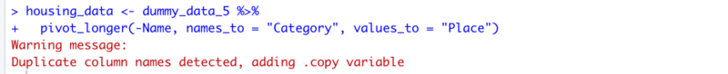
The resulting output looks cleaner.

The copy column tells you about the number of different copies of the same type of data.

Multiple observations per row (Hard Example)

Those who are already fed up with pivoting can skip this special case but there might be a case when a single row might contain data corresponding to multiple observations.

So far, we have seen data frames with one observation per row. Even in the multiple variable example we have just 1 observation. Multiple observations can be recognised by having the same substring re-appear in the names of multiple columns.

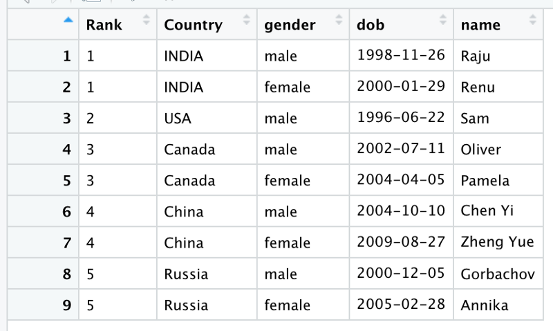
Let’s take a look at an example. The 4th dummy dataset contains information about the athletes who won in the Olympics. Each row contains country’s name, the date of birth of its top male and female athletes and their names.

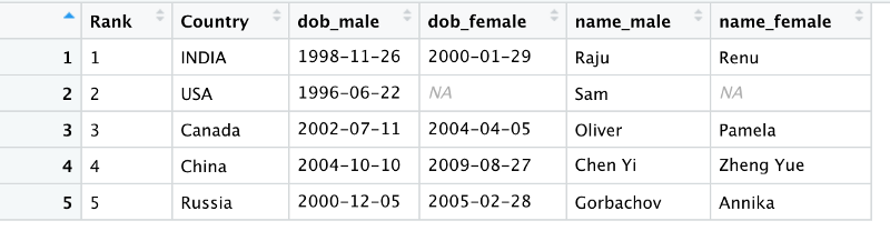
Note that we have 2 observations per country

1. DOB and Name for the male athlete
2. DOB and Name for the female athlete

Both of these need to go into separate columns in the resulting data frame. We will again usenames_sep to split up each variable name. Let’s try pivoting this

winner_data <- dummy_data_4 %>% 
  mutate_at(vars(starts_with("dob")), parse_date) %>%
  pivot_longer(
    cols = -c(Rank,Country), 
    names_to = c(".value", "gender"), 
    names_sep = "_", 
    values_drop_na = TRUE
  )

• Note the special name .value ; this tells pivot_longer()that anything that comes before the separator (names_sep) is to be picked up as a column name
• gender containes anything after the separator as column values
• So, the column names dob_male, dob_female, name_male, name_female contain the words male and female after the separator and these go into the Gender column as values.
• mutate just changes the type of the column dob from string to date

Pivoting is immensely useful when piping data as well for plotting. It helps in a better data analysis and a cleaner representation. There are times though when we might want to switch back to a wider format. In the next article we will take a look at how to pivot back from longer to the wider form.

Special thanks to Rahul for introducing me to R and getting me up to speed with the beauty of pivoting. Also, thanks to him for editing this article.