Becoming an Expert at Joins in R
Data in the real world exists as a collection of distinct information. More often than not this information is organised as tables. Each table collecting data on a different aspect of the ecosystem. For example, a school might organise its data into the following tables
- Teacher information
- Student attendance
- Student marks
- Salary information, etc…
We can clearly see that tables 2 and 3 will have something in common (student IDs for one), just like tables 1 and 4 (teacher IDs for instance).
Such overlap of information across tables is quite common and becomes the basis for a join. A join lets you combine information from different tables. In R we have 6 types of joins. Let’s explore each of them with an example. But first let’s look at the data we are going to be working with.
Dummy Data
We will visit the world of Hogwarts and pick up some data.
library(dplyr)citizen_df <- tribble(  ~Person, ~Citizenship,  "Harry",   "UK",  "Harry",   "USA",  "Ron",   "India",  "Ron",   "Pakistan",  "Hermoine",   "UK",  "Hermoine",   "USA",  "Hermoine",   "Russia",  "Dumbeldore", "Poland",  "Dumbeldore", "Singapore")
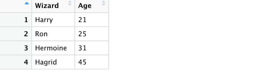
age_df <- tribble( ~Wizard, ~Age, "Harry", 21, "Ron", 25, "Hermoine", 31, "Hagrid", 45)Age Data
Let’s get some wizards’ and witches’ age data.
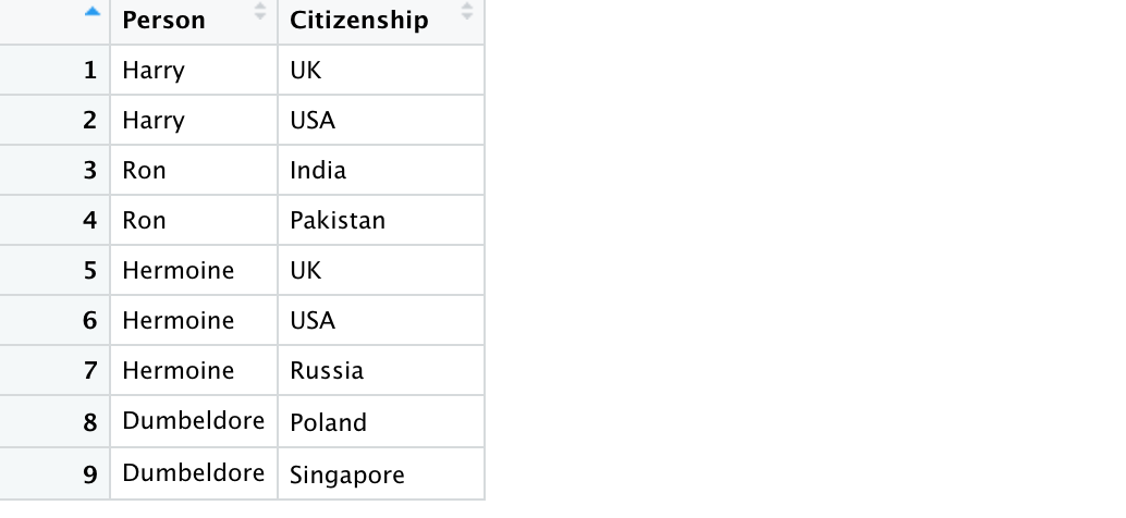
Citizenship Data
Let us also figure out their citizenship status.
Joins
We will explore the following joins
- Inner Join
- Left Join
- Right Join
- Full Join
- Anti Join
- Semi Join
When we join a table X with a table Y there needs to be a column that is common to both. This is called the key by which the two tables are joined. Based on this key column we join the two tables. For example in the wizard data above both tables contain a column that contains the names of the wizards. In the age table it is called wizard column and in the citizenship table it is called the person column. Let’s see how to join.
Inner Joins
Inner join is the most commonly used join. It keeps those rows which contain data that is common to both the tables. e.g. if we perform an inner join on the above two tables we will loose the rows containing Hagrid and Dumbeldore.
Diagrammatically, it looks like this. Note that the final table contains 3 columns instead of two but preserves only the common rows.
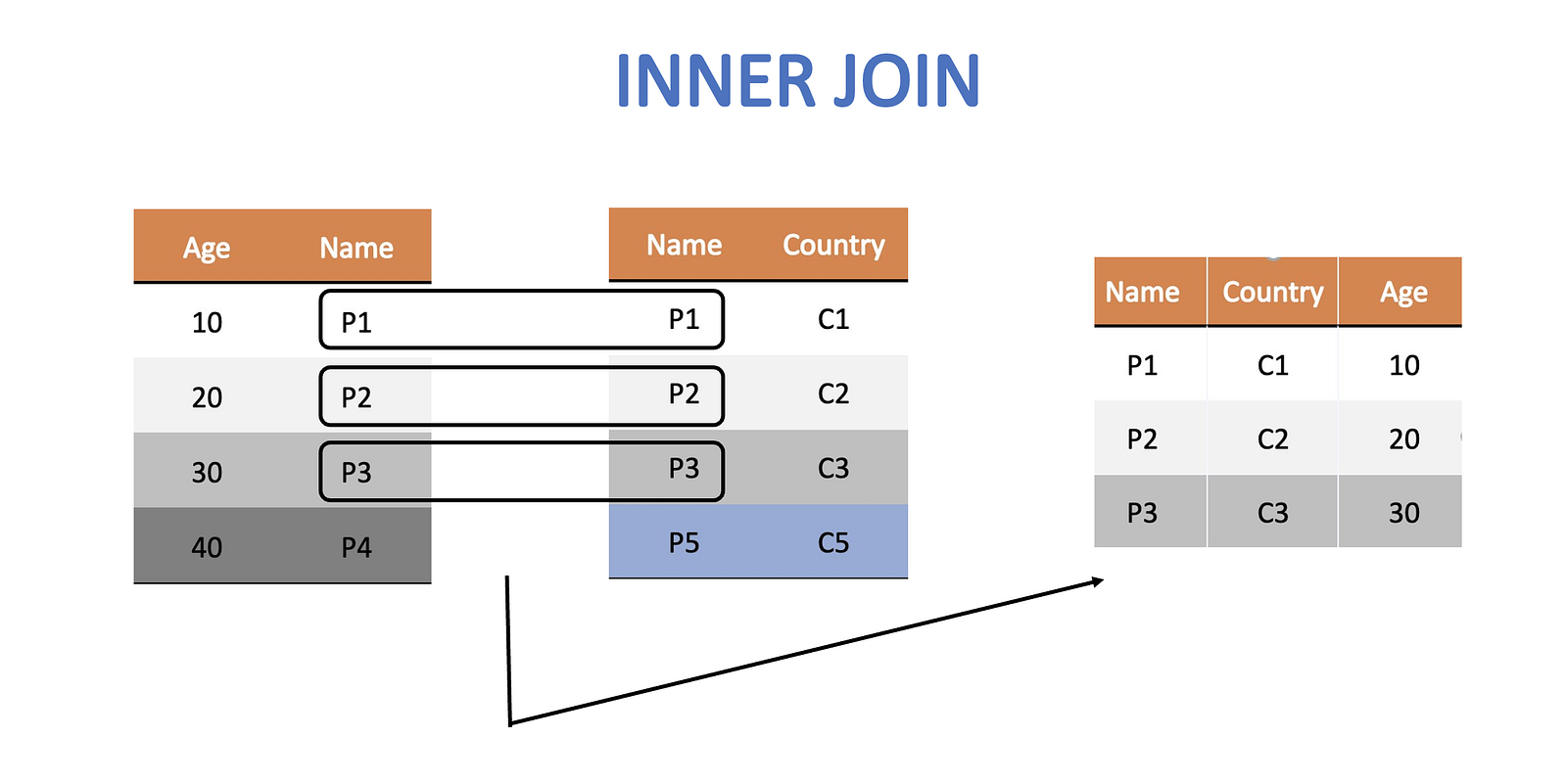
After the join we can easily identify both the age and citizenship of our wizards and witches from the same table.
Let’s code this up. Note the use of by(), which is done to explicitly specify the column that is common to both the tables. This is essential if the common column has different names in the two tables.
inner_join_df <- inner_join(age_df, citizen_df, by = c("Wizard" = "Person")) 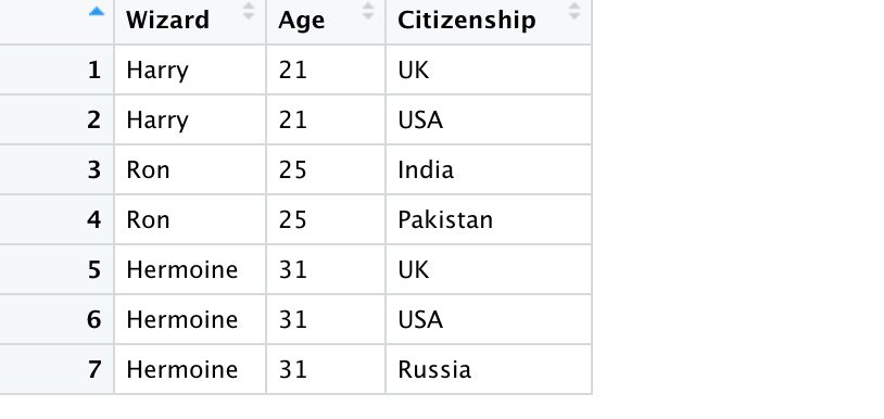
Outer Joins
There are 3 types of outer joins — left, right and full join. An inner join keeps information that is common to both the tables, but an outer join retains information that appears in at least one of the two tables. In that sense, they are akin to intersection and union respectively.
Left Join
The left join keeps all the rows of the left table. If it is unable to find a corresponding row in the right table then it fills it as NA.
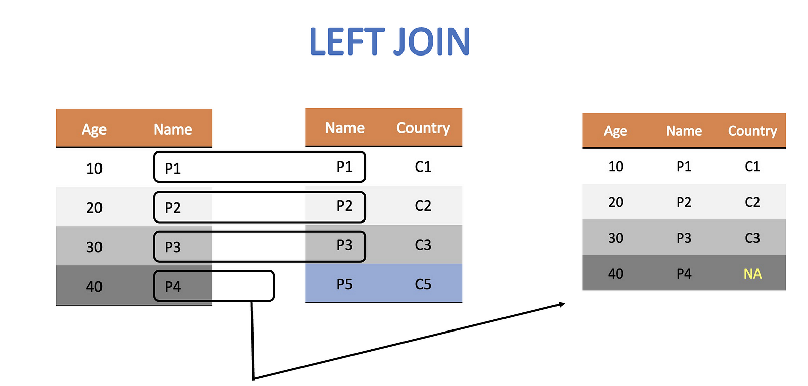
left_join_df <- left_join(age_df, citizen_df,by = c("Wizard" = "Person"))
Notice how Hagrid is left without any citizenship information as the right table has no row corresponding to Hagrid.
Right Join
Similarly, the right join keeps all the rows of the right table. If it is unable to find a corresponding row in the left table then it fills it as NA.
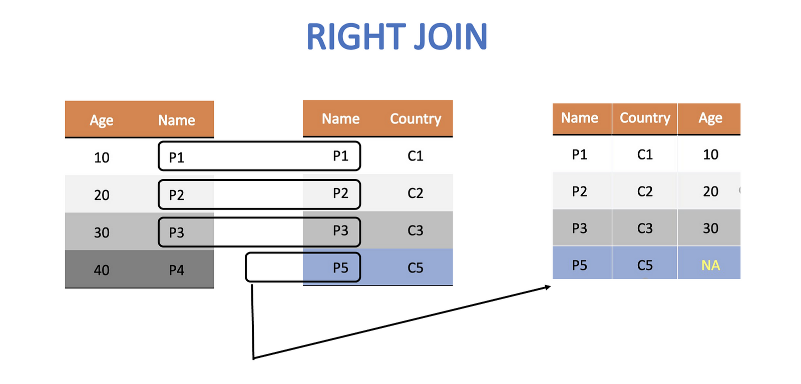
right_join_df <- right_join(age_df, citizen_df, by = c("Wizard" = "Person"))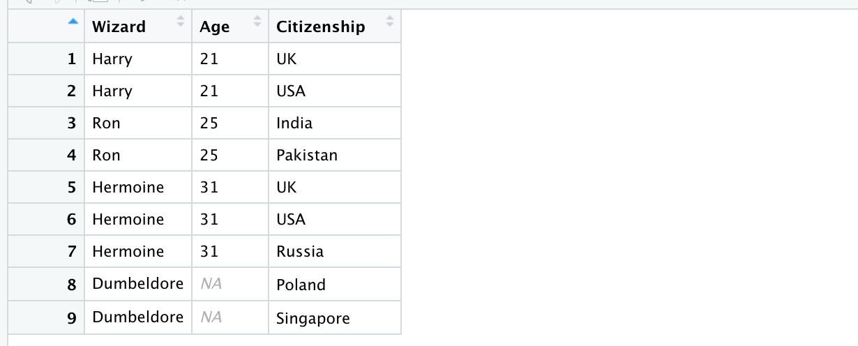
Notice how it is Dumbeldore this time who is left without any age information as the left table has no row corresponding to him.
Full Join
A full join keeps all rows from both the tables. Consequently, it is bound to have many NAs if there is missing information.
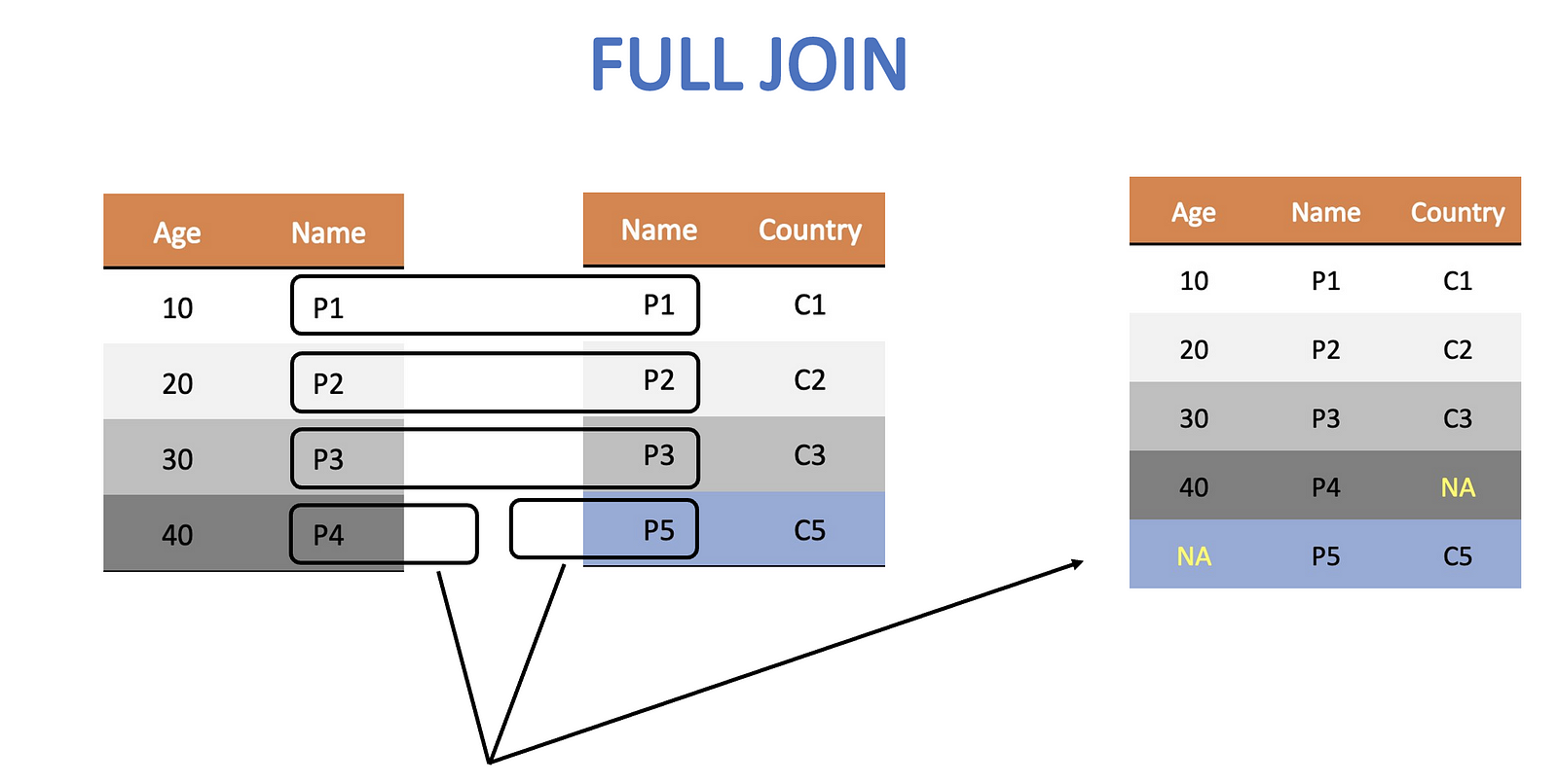
The code for it is
full_join_df <- full_join(age_df, citizen_df, by = c("Wizard" = "Person"))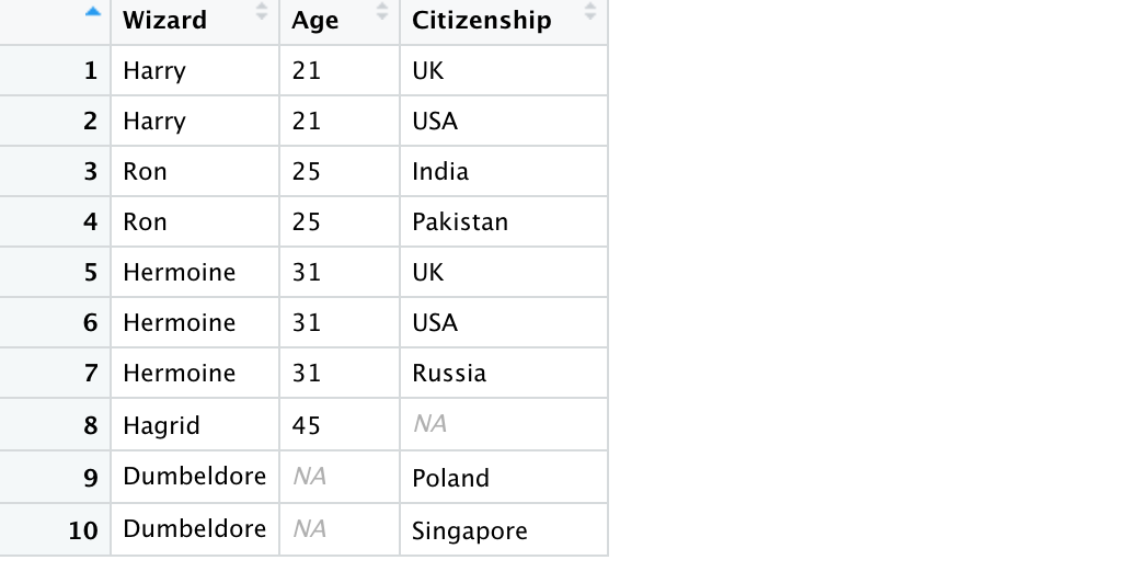
Filtering Joins
Filtering joins do not combine information from the two tables. They just keep information of the left table but filter it based on what is found in the right table. The two types of filtering joins we will talk about are — anti join and semi join
Anti Join
Anti join gets rid of all rows in the left table that have a presence in the right one.
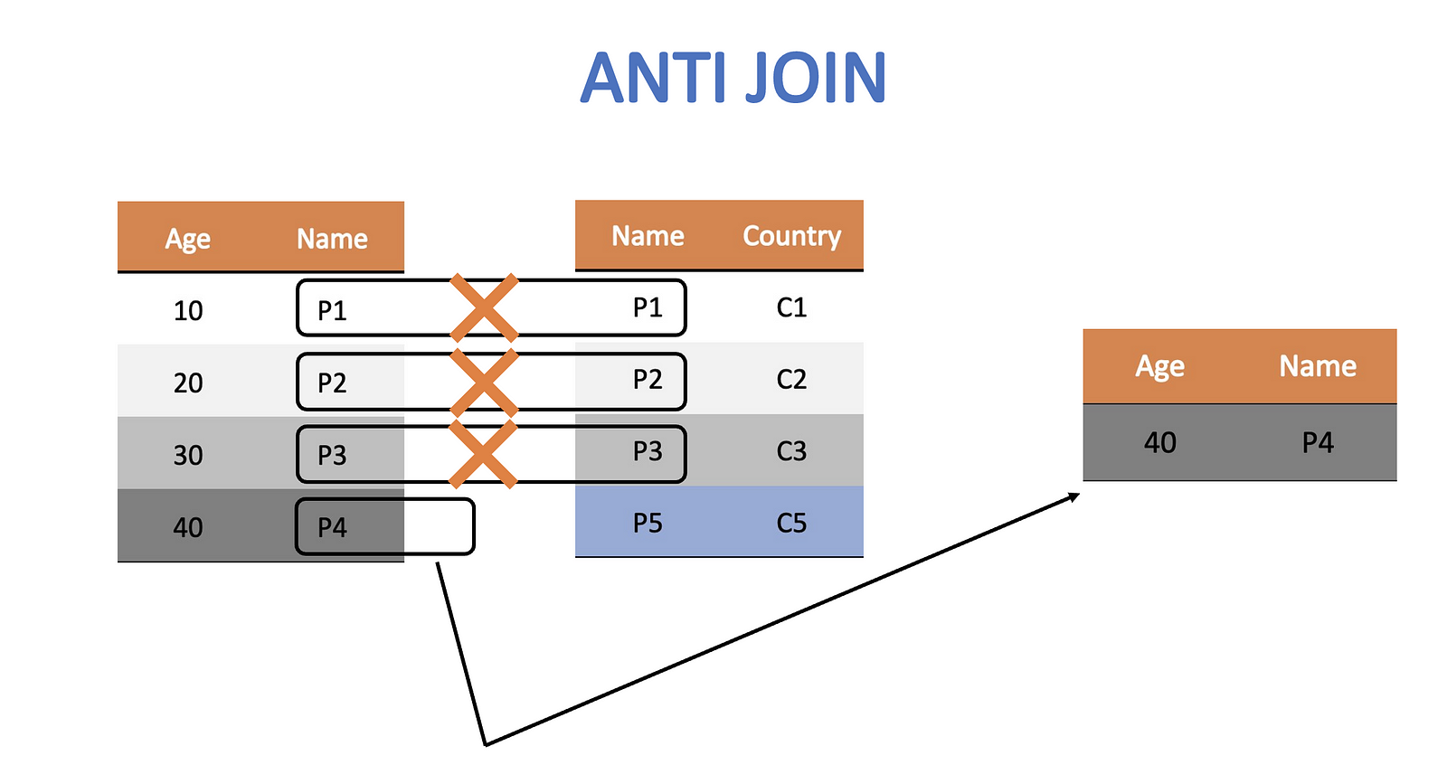
anti_join_df <- anti_join(age_df, citizen_df,by = c("Wizard" = "Person"))
Note how we do not have any citizenship information in this final table. The reason is that filtering joins do not combine information. They only filter.
Semi Join
It is the opposite of an anti join. Semi join gets rid of all rows in the left table that do not have a presence in the right one.
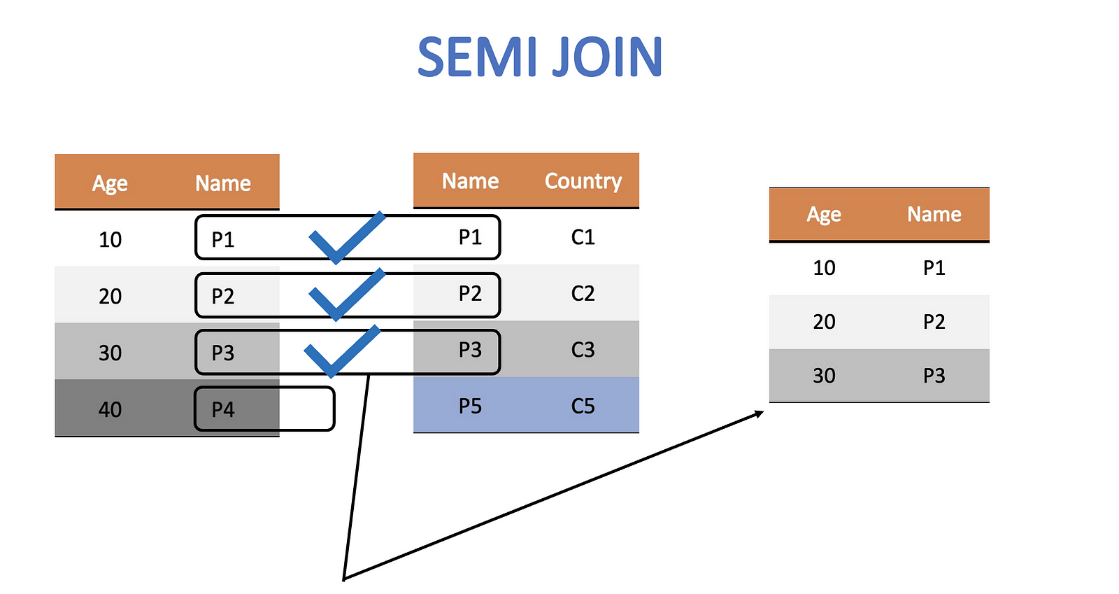
semi_join_df <- semi_join(age_df, citizen_df,by = c("Wizard" = "Person"))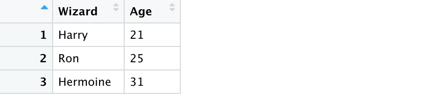
Visualising Joins
Most join diagrams show them as venn-diagrams. While conceptually we can show inner join to be similar to intersection there are subtle differences that do not convey the complete picture. I find the analogy of a cross-product closer to the actual meaning of a join. Let’s take a look at an example.
Data
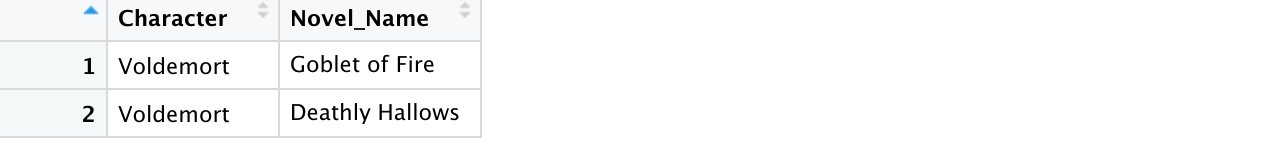
Let’s say we have 2 tables containing the kills-information and the information about which character appeared in which novel. Each table has multiple rows containing Voldemort. This means that the key has duplicate entries.
kills_df <- tribble(  ~Killer, ~Killed,  "Voldemort",   "Cedric",  "Voldemort",   "Snape",)
appearance_df <- tribble(  ~Character, ~Novel_Name,  "Voldemort",   "Goblet of Fire",  "Voldemort",   "Deathly Hallows",)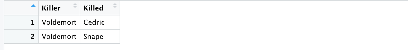
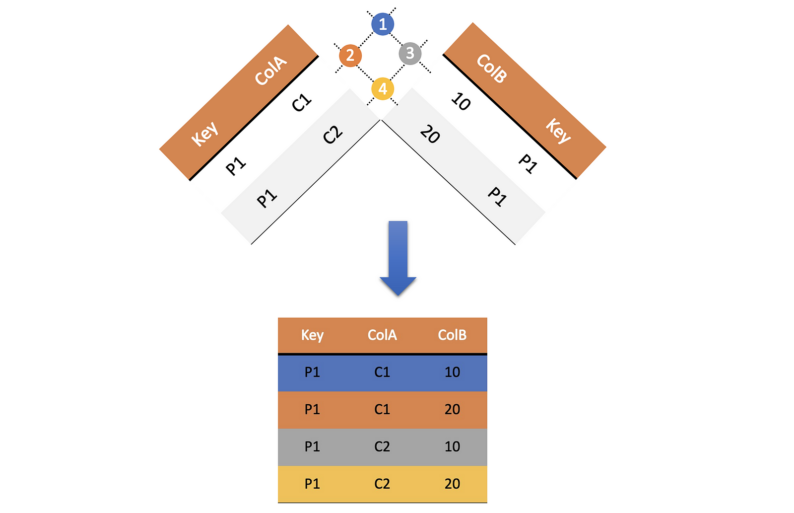
Join as a cross product
Now we will attempt a left-join on these two tables. What do you think the resulting table looks like.
cross_left_join_df <- left_join(appearance_df, kills_df,by = c("Character" = "Killer"))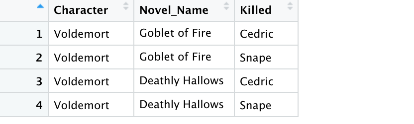
The output contains all possible combinations of the rows, much like a cross product.
Joins are widely used in databases. R provides very neat commands to execute these nifty instructions. These go a long way in furthering your career as a backend developer.
Member discussion