Jun 3, 2020 5 min read R

'Rock'ing Analysis in R

Extracting insights from the data of top 500 music albums of all time.

Rolling Stones’ list of top 500 Albums is considered by many as the compilation of best music ever. As a beginner in R, I started to look at this dataset with the help of Rahul and Rishi Sidhu.

Let us look at the dataset and see what insights we can get from it.

# Load datamusic <- read.csv( "https://query.data.world/s/nk72czqmyopg254j245xl7dss7xdjm", header=TRUE,     stringsAsFactors=FALSE    )

#get dimensions of data
dim(music)
[1] 500 6

The dataset has 500 rows and 6 columns. The dataset looks like this:

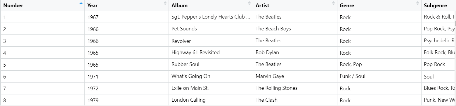
We have top 500 albums with their ranks (Number), Artists and Genres. Let us first analyze year-wise distribution to understand which is/was the golden era of music.

p <- ggplot(data = music, aes(x = Year)) +  
     geom_bar() +  
     theme_minimal()
print(p)

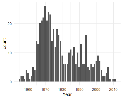
We can see that 70’s was the golden era of music. We could also populate the bars for each year with each genre or artist. Note the use of ‘fill’ argument in the aesthetic.

#some values in genre includes multiple genres. So separate by default
#delimitier to get single value in 'Genre' column
d_music <- music %>% 
  separate(Genre, c('Genre') )

p <- ggplot(data = d_music, aes(x = Year, fill = Genre)) +   
 geom_bar() +  
 theme_minimal()

print(p)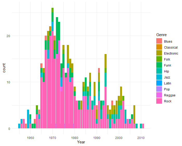

We can see that Rock (pink color) was the predominant genre in 70's

Now let’s try to find the most successful artist in this list. Success can be subjective. So you could find any metric to define it. For the sake of simplicity, I will focus on the top 100 albums only. Smaller the ‘Number’, better the rank of the album. Another important parameter of success could number of times an artist is featured in top 100.

d_threshold <- 100
d_artist_100 <- music %>%  
  mutate(Number_thre = ifelse(Number > threshold, 0, threshold -                  Number)) %>%  
  filter(Number_thre  > 0) %>%  
  group_by(Artist) %>%   
  mutate(Number_of_Features = n()) %>%  
  ungroup()

In the above code,

mutate creates a new column Number_thre which takes a value of 0 if Number is greater than 100, else it is 100 — Number.
filter function keeps only those rows for which Number_thre > 0 i.e. album rank is above 100.
Finally, we group the dataframe by Artist and then calculate a new field Number_of_Features in top 100.

If you are new to use of piping (%>%) in R, here is a very informative article.

This is how the resulting dataframe looks:

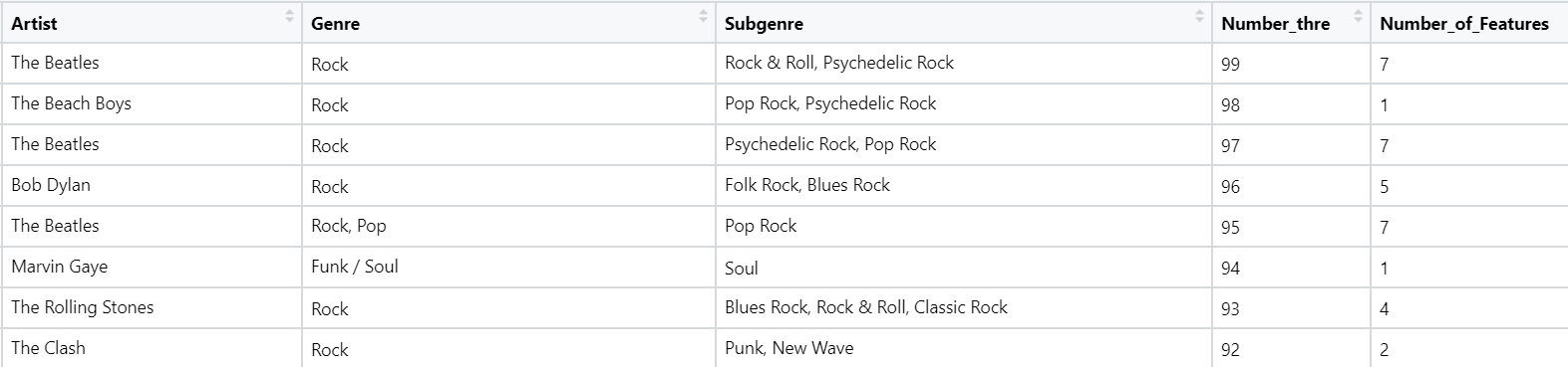
Looking at the dataframe, we can see that there are a lot of artists which are featured only once in the top-100 while there are some which have repeated features. For finding most successful artists, we only keep artists with 1 or more features. A simple way of ranking the artists can be taking mean of their Ranks which we just calculated.

d_artist_100 <- d_artist_100 %>% 
  group_by(Artist) %>%  
  filter(Number_of_Features > 1) %>%   
  summarize(Ranking = sum(Number_thre)/mean(Number_of_Features))  %>%  
  ungroup()

#order them based on Ranking
d_ranked <- d_artist_100[order(d_artist_100$Ranking),]

# we use tail for showing top high ranks
tail(d_ranked)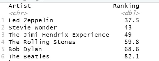

To see this visually, let’s plot it.

plt = ggplot(data = d_ranked, aes(x = Artist, y = Ranking, fill =              Ranking)) +   
     theme(axis.text.x = element_text(angle = 45, hjust = 1)) +  
     geom_col(aes(reorder(Artist,Ranking),Ranking))   

print(plt)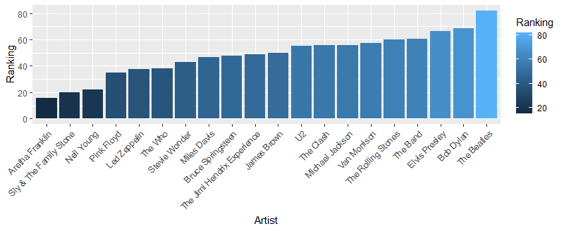

Now let’s see how versatility of an artist correlates with their success. We can define versatility as the number of genres they have explored. Within the limits of this dataset, let’s explore this:

First, we will separate genre and subgenre columns in the original dataframe into a number of genres. This can be achieved using separate function as seen previously. We want to get this data in long format, as we want to count the number of genres for each artist. Learn more on pivoting in this article.

Now we can group by Artist and count distinct genres. Multiple albums can have same genre and hence we need to find distinct genres.

p_genre <- music %>%   
 separate(Genre, c('Genre1', 'Genre2', 'Genre3'), sep = "([\\,\\&])") %>%   separate(Subgenre, c('Genre4', 'Genre5', 'Genre6'), sep ="([\\,])") %>% 
  pivot_longer(-c(Year, Album, Artist, Number), values_to ="Genre",        values_drop_na = TRUE) %>%  
  group_by(Artist) %>% 
  summarize(NGenre = n_distinct(Genre)) %>%  
  ungroup()

Now we have list of Artists and Number of genres. Previously, we created another dataframe d_ranked which had list of artists and their ranking. Let’s join the two data frames. Function inner_join takes two dataframes and joins them based on common key Artist. Let us also see how the joined dataframe looks.

p_genre <- inner_join(p_genre, d_ranked, by = c("Artist" = "Artist") )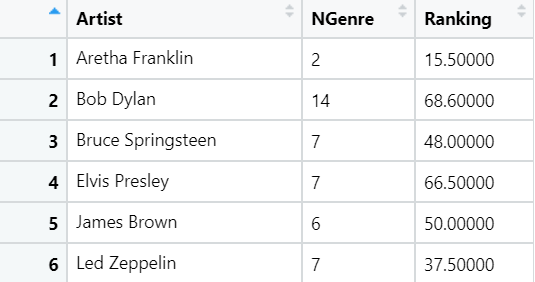

Now let’s plot this data to visually see this correlation. Some point to note are: we want to plot a dot (point) graph and we want the size of dots proportional to ranking. We would like to annotate the dots with names of artists: geom_label_repel in ggrepel package provides a clean way to do that.

plot_corr = ggplot(p_genre, aes(x = NGenre, y = Ranking)) +   
  geom_point(aes(size = Ranking, colour = factor(Ranking)), show.legend = FALSE) + 
  xlab('Number of Genres') + 
  ylab('Awesomeness') +  
  theme_minimal() +  
  geom_label_repel(data= p_genre, aes(x=NGenre, y=Ranking, label=Artist))

print(plot_corr)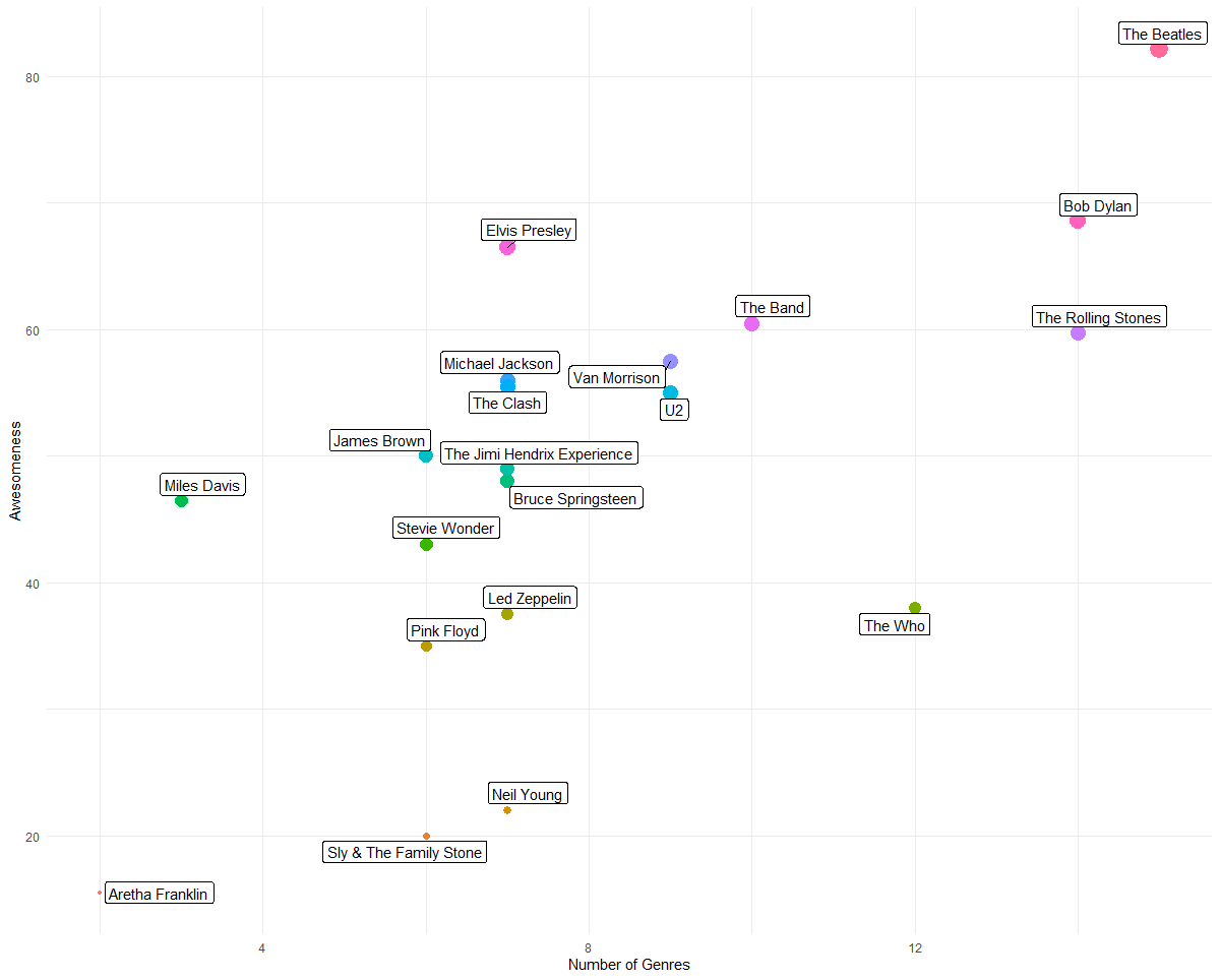

We can do a lot of more with this dataset. To see, which artists rocked decadewise or which artists succeeded for many decades. If you are interested in this analysis, feel free to reach out for the code. Have fun with R.

Thanks to Rahul and AI Graduate Admin for helping me learn this. For more fun assignments in R, do follow this Github repo made by Rahul.