Decision Tree Visualisation — Quick ML Tutorial for Beginners

A 10 line python code for beginners to construct a decision tree and visualise it

Twenty questions is a game that essentially lets you guess the answer by asking 20 yes/no questions. Decision tree is an algorithm that works on the same principle. It is a machine learning methodology that lets you decide the which category does the object in question belong to, based on a series of questions.

A very nice article by Prateek Karkare expounds on the intuition behind this algorithm. Let us see how to code it up.

Decision Trees — An Intuitive Introduction

Shopkeeper asks,“How can I help you Ma’am?”“I am looking for a cell phone”“You are at the right place, we have over 300 different types of cell phones, what kind of phone would you like to buy…

AI GraduatePrateek Karkare

Dataset

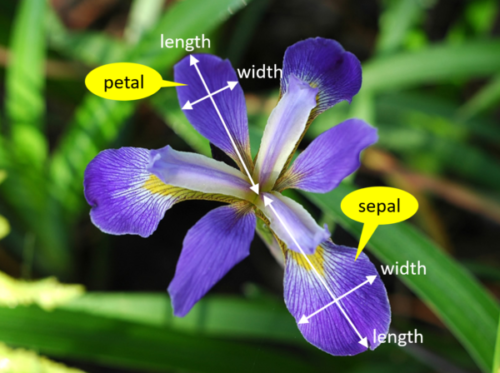
We are going to use the Iris flower dataset. This data set lists a few features — sepal and petal lengths, and widths — of 3 different types of iris flower. What we want to do with decision tree is to differentiate these 3 types of iris — Iris Setosa, Iris Versicolor and Iris Virginica — based on the features.

The features that we have for each of these types of iris are going to help us differentiate between them. For example, from the images above we can clearly see that the Virginica petals are much wider than Setosa petals and a quick look at the data corroborates that observation.

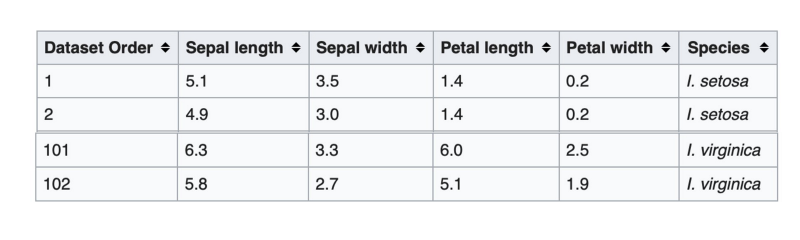
Wikipedia mentions the complete details of the data set. One can go over there and study the dataset in depth. All we need to start coding is that there are 150 rows in the dataset, 50 per type of iris.

• Class 0 stands for Setosa and takes up rows 0–49
• Class 1 stands for Versicolor and takes up rows 50–99
• Class 2 stands for Virginica and takes up rows 100–149

Now let’s start building the code needed for constructing our decision tree.

Code Walkthrough

1) Loading and taking a peek at the data

Let’s load the data into the memory, look at the features and print a few examples of each class of flower.

from sklearn.datasets import load_iris
iris = load_iris()
#Print Feature Names
print("Feature Names - ", iris.feature_names,"\n")

#Print the row 0,50 and 100 i.e. 1 example for each type
print("\nSetosa flower 1 - ",iris.data[0])
print("Versicolor flower 1 - ",iris.data[50])
print("Virginica flower 1 - ",iris.data[100],"\n")

This matches with the wikipedia screenshot pasted in the dataset section above.

2) Splitting the dataset

In any machine learning algorithm we need to train the model on a set that is very different from the dataset on which it is tested. So we will split our dataset into two parts.

import numpy as np
#Choose top 2 examples of each flower type as test rows
test_indices = [0,1,50,51,100,101]

#training data
train_target = np.delete(iris.target, test_indices)
train_data = np.delete(iris.data, test_indices, axis=0)

#testing data
test_target = iris.target[test_indices]
test_data = iris.data[test_indices]

3) Training and testing the decision tree classifier

We will use Python’s sklearn library to build a decision tree classifier

from sklearn import tree

#Build the classifier
dtClassifier = tree.DecisionTreeClassifier()

#Train the classifier
dtClassifier.fit(train_data, train_target)



#Print the actual labels of each test point
print("\n********** Actual **************")
for p in range(len(test_indices)):
 print("Test Row ",test_indices[p], " belongs to the class ",test_target[p] )

predicted_target = (dtClassifier.predict(test_data))

#Print the predicted labels of each test point
print("\n********** Predicted **************")
for p in range(len(test_indices)):
 print("Test Row ",test_indices[p], " is predicted to be of the class ", predicted_target[p] )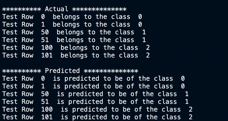

4) Visualising the tree

We will use the graphviz library to visualize the tree. macOS users will have to install graphviz using homebrew, just pip install won’t do.

#Visualize The Decision Tree
from graphviz import Source
graph = Source(tree.export_graphviz(dtClassifier, out_file=None, 
                     feature_names=iris.feature_names,  
                     class_names=iris.target_names,  
                     filled=True, rounded=True,  node_ids= True,
                     special_characters=True))
graph.format = 'png'
graph.render('dtree_render',view=True)

Observe how at each node of the tree one has to make a decision and then move left or right based on the answer. Node 0 checks whether petal width is ≤ 0.8 cm. If that is true the flower is cateogrized as a Setosa right away. Otherwise, we go to node 2 and check if petal width ≤ 1.75cm and so on.

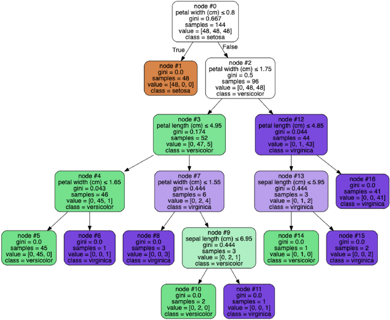
Take a look at an actual test row being run through a decision tree. The example row in question is Row 100 of the class Virginica.

You can try running an example of your own through the tree and see if it works for you.

Next Steps

A single decision tree by itself is not immensely useful. It is quite error prone and unreliable to have just a single decision tree. Rather, a more practical use case of decision trees is to use a lot of them. That is called a random forest. This article goes into the intuitive understanding behind random forests. In the future, we will build a similar code walkthrough for a random forest as well.

AI Graduate aims to organize and build a community for AI that not only is open source but also looks at the ethical and political aspects of it. More such experiment driven simplified AI concepts will follow. If you liked this or have some feedback or follow-up questions please comment below.