Beginner’s Introduction to Matrices

Matrix operations are being used everywhere from theoretical physics to neural networks.

Matrices are the building blocks of data science. They appear in various avatars across languages. From numpy arrays in Python, to dataframes in R, to matrices in MATLAB.

The matrix in its most basic form is a collection of numbers arranged in a rectangular or array-like fashion. This can represent an image, or a network or even an abstract structure.

Matrices, plural for matrix, are surprisingly more common than you would think.

All our memes that get made through Adobe Photoshop use matrices to process linear transformations to render images. A square matrix can represent a linear transformation of a geometric object.

For example, in the Cartesian X-Y plane, the matrix

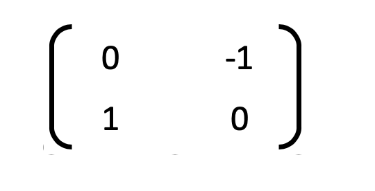
is used for creating the reflection of an object in the vertical Y-axis. In a video game, this would render the upside-down image of an assassin reflected in a pond of blood. If the video game had curved reflecting surfaces, such as a room of mirrors, the matrix would be more complicated, to stretch or shrink the reflection.

In applied physics, matrices are used to study electrical circuits, quantum mechanics and optics. Aerospace engineering, chemical engineering, etc. all require perfectly calibrated computations which are obtained from matrix transformations. In hospitals, medical imaging, CAT scans and MRI’s, use matrices to generate the outputs.

In programming, matrices and inverse matrices are used for coding and encrypting messages. In robotics and automation, matrices are the basic components for the robot movements. The inputs for controlling robots are obtained based on the calculations using matrices.

What do they look like?

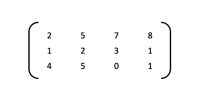
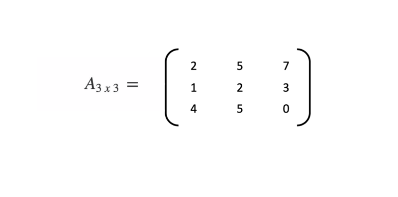
Conventionally, the number of rows in a matrix is denoted by m and the number of columns by n. Since a rectangle’s area is height x width, we denote a matrix’s size by m x n. Thus is the matrix was to be called A, it would be written notationally as

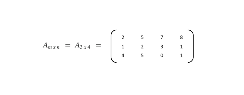
Here m=3 and n=4. Thus there are 12 elements in the matrix A. A square matrix is one which has m=n.

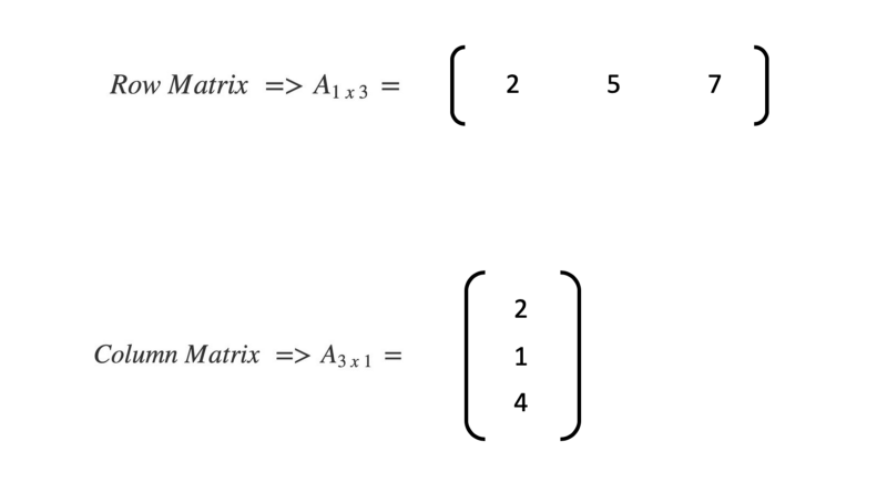
A matrix with just one row is called a row matrix and a matrix with just one column is called a column matrix.

What can we do with them?

Matrices just like numbers can be added, subtracted and multiplied. The division though is slightly nuanced. Not all matrices can be divided.

There are certain rules for even the addition, subtraction and multiplication.

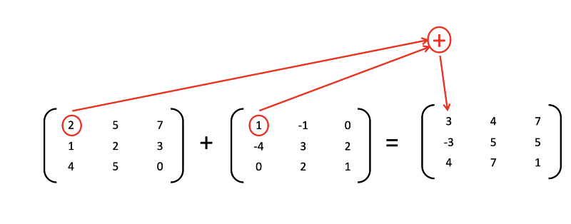
Matrices Addition

The addition of two matrices A(m*n) and B(m*n) gives a matrix C(m*n). The elements of C are the sum of corresponding elements in A and B

Subtraction works similarly.

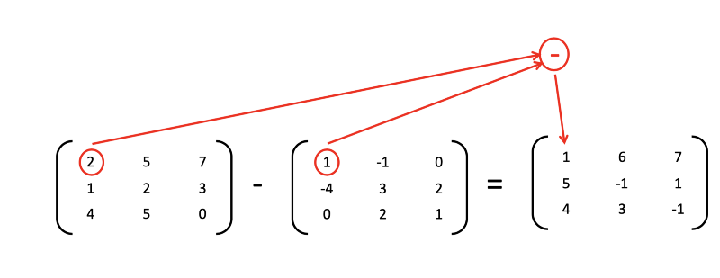
The thing to note here is that you can only add/subtract matrices with the same number of rows and columns i.e. the same order (order = rows x columns)

• Number of Rows of A = Number of Rows of B
• Number of Columns of A = Number of Columns of B

Points to note

• Addition of matrices is commutative which means A+B = B+A
• Addition of matrices is associative which means A+(B+C) = (A+B)+C
• Subtraction of matrices is non-commutative which means A-B ≠ B-A
• Subtraction of matrices is non-associative which means A-(B-C) ≠ (A-B)-C
• The order of matrices A, B, A-B and A+B is always the same
• If the order of A and B is different, A+B, A-B can’t be computed
• The complexity of addition/subtraction operation is O(m*n) where m*n is order of matrices

Multiplication though is slightly complicated

Matrices Multiplication

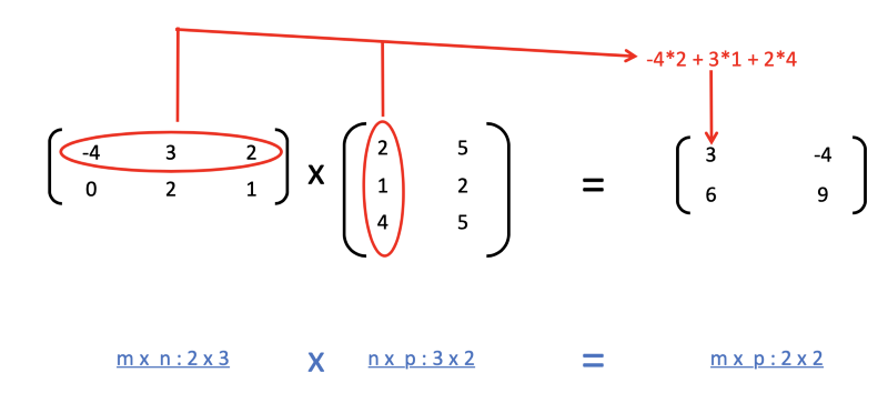
The multiplication of two matrices A(m*n) and B(n*p) gives a matrix C(m*p). Notice that for multiplication you do not need the rows/columns of A and B to be the same. You only need

• No. of Columns of A = No. of Rows of B
• Or, No. of Columns of B = No. of Rows of A.

To calculate the top-left element of the resulting matrix C, multiply elements of 1st row of A with 1st column of B and add them

Points to note

• Multiplication of matrices is non-commutative which means A*B ≠ B*A
• Multiplication of matrices is associative which means A*(B*C) = (A*B)*C
• Existence of A*B does not imply the existence of B*A
• The complexity of multiplication operation (A*B) is O(m*n*p) where m*n and n*p are an order of A and B respectively
• The order of matrix C computed as A*B is m*p where m*n and n*p are order of A and B respectively

In the next edition of this article, we will see more operations that can be performed on matrices e.g. Inverse of a matrix, determinant of a matrix, adjoint of a matrix, etc.

We will also see how these matrices actually help in the field of neural networks and image processing.

Matrices are of huge importance in almost all of the machine learning algorithms from KNN(K -Nearest Neighbor algorithm) all the way to Random Forests.