Handling Matrices in Python — A NumPy Tutorial

NumPy provides Python users with the ability to manipulate matrices — a much needed thing for AI

Traditionally MATLAB has been the most popular matrix manipulation tool. NumPy gives python users the same super power and with that it makes it easy for them to perform neural network calculations and numerous other AI tasks.

Machine learning is built on top of mathematics. The most commonly used data structure in machine learning is a matrix. Go here if you want a quick introduction to matrices.

Matrices occur when you want to compute activations of neurons in a neural network. They occur when computing reflections in a video game. Let’s see how to work them with NumPy.

Numpy is the core library for scientific computing in Python. It provides a high-performance multidimensional array object, and tools for working with these arrays.

The name is an acronym for “Numeric Python” or “Numerical Python”. It provides various functionalities like creating arrays, adding them, multiplying them and even taking their transpose and inverse. The theory behind these terms can be found here.

In python, as in most other languages, a matrix is called an array

Array Creation

Let’s start by looking at how to create an array. This is an array with 3 rows and 3 columns

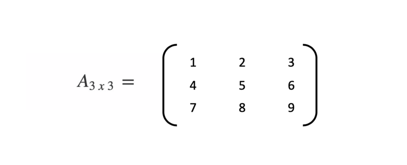
To create this array in numpy we would need to do this

import numpy as np
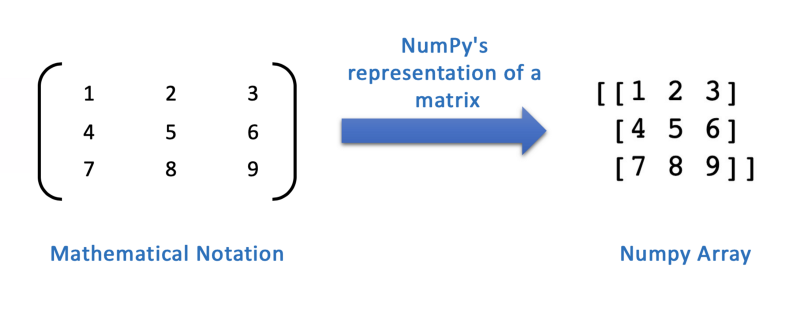
A = np.array([[1,2,3],[4,5,6],[7,8,9]])
print(A)

So we can see how mathematical notation of a matrix is represented in NumPy. Every row is enclose within square brackets and finally the whole array is enclosed within a set of brackets

Sometimes one needs to initiate a zero matrix or a unity matrix. Let’s say we want to print a matrix of zeros with 2 columns and 3 rows

A = np.zeros((3,2))
print(A)

Let’s look at a few more types of matrices namely — ones, identity, constant and random

A = np.ones((3,2)) #Matrix of all 1's
print(A)

B = np.identity(3) #Identity Matrix
print(B)

C = np.full((2,2), 5)  # Create a constant array
print(C)               # Prints "[[ 5.  5.]
                       #          [ 5.  5.]]"
R = np.random.random((3,3))  # Create an array filled with random values
print(R)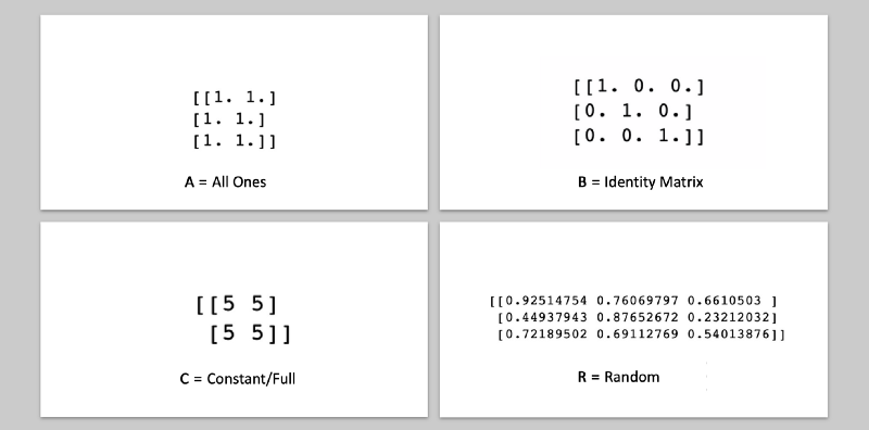                     

Array Indexing / Slicing

Oftentimes you need to extract a subset of an array. You need only a few elements from that array. This operation is called array indexing. Slicing is another term used to cut an array’s portion out of it

Let’s create a row matrix first and select a few elements in it. The first thing to observe is that when we start counting an array’s elements in python we start from 0. So the first element is at the 0th position. To select that element we write A[0]. Also observe we use a new method to create a new matrix called arange. It creates a row matrix of integers starting from 0 to 1 less than the number we pass as an argument to arange.

A = np.arange(10)
print("A    = ", A)   # [0,1,2,3,4,5,6,7,8,9]
print("0th  = ",A[0]) # Will output the 1st element
print("8th  = ",A[8]) # Will output the 9th element
print("-1th = ",A[-1])#Guess?

A[-1] interestingly gives us the 1st element from last. Let’s see how to get more than one elements from the array. Guess what each print statement will output before looking at the answers below.

#Select elements from 0th position to 3rd position
print("A[0:4]    = ", A[0:4])

#Select elements from -3th position to 2nd last position
print("A[-3:-1]  = ", A[-3:-1])

#Select every 2nd element from 0th to 10th position
print("A[0:10:2] = ", A[0:10:2] )

#Another way of writing the above
print("A[:10:2]  = ", A[:10:2] )   

#Select every 2nd element from 1st to 10th position
print("A[1:10:2] = ", A[1:10:2] )  

#Modify every third element
A[:10:3] = 38
print("A         = ", A)

But this is just a row-matrix i.e. a one dimensional array. Let’s create a 2-dimensional array. Pay attention to how we create this one. We create a row array and keep reshaping it to make a 2D matrix until we convert it into a column matrix.

#Create a row matrix
B = np.arange(12)
print("B   = ",B)

#Reshape it to have 3 rows and 4 columns
C = B.reshape((3,4))
print("C   = \n", C)

#Reshape it to have 4 rows and 3 columns
D = B.reshape((4,3))
print("D   = \n", D)

#Reshape it to have 6 rows and 2 columns
E = B.reshape((6,2))
print("E   = \n", E)

#Reshape it to make a column matrix
F = B.reshape((12,1))
print("F   = \n", F)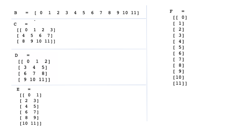

Now let’s select a few elements from C array.

#Slice out the first 2 rows and the first 3 columns from C
print(C[0:2,0:3])

#Slice out the first 2 rows and all columns from C
print(C[0:2,:])

#Slice out just first row
print(C[0,:])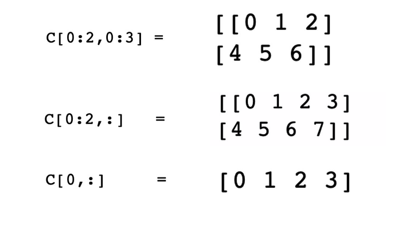

Array Transformations

Before we can proceed to performing addition, subtraction and multiplication we might need to transform the array in some way. The reshape method above is one such transformation. Let’s look at a few others

# Original Array
print("C   = \n", C, "\n")

# returns the array, flattened
print("Flattened C = \n", C.ravel(),"\n")

#Transpose of C
print("Transpose of C = \n", np.transpose(C),"\n")

# Inverse of a slice of C (why can't we take C's inverse?)
np.linalg.inv(C[1:3,1:3])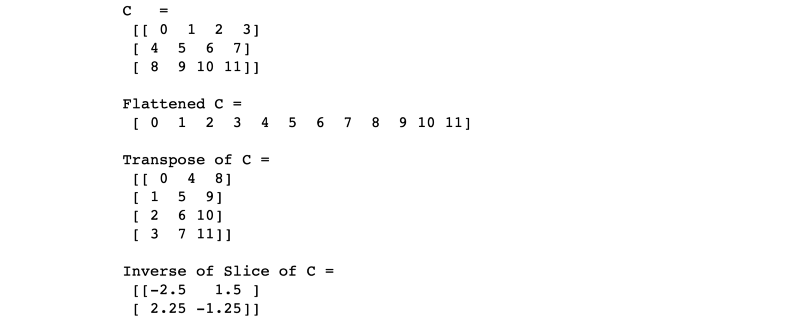

Note that we had to take a slice of C before taking inverse? If you go back to the basics of matrices part II you will remember that we can take inverse of a square matrix only and that too should be non-singular (i.e. it’s determinant should be non-zero).

If we try to take inverse of C what do we get?

np.linalg.inv(C)

Mathematical Operations

Finally let’s look at what kind of mathematical operations can we do with numpy array.

#original array
A = np.array([[1,2],[2,1]])

#Double each element of array A
B = A*2

#Add 2 to every element of array A
C = A + 2

#Add A to B
D = A+B

#Add A to B to C
E = D + C

#Print all of them
print("A = \n",A,"\n")
print("B = \n",B,"\n")
print("C = \n",C,"\n")
print("D = \n",D,"\n")
print("E = \n",E,"\n")

Let’s try a few other operations

#Element wise multiplication
F = np.multiply(A,B)
#Matrix Multiplication
G = np.dot(A,B)
#Sum all elements of a matrix together
H = np.sum(A)
#Sum all elements along row direction
I = np.sum(A, axis = 0)
#Sum all elements along column direction
J = np.sum(A, axis = 1)

print("F = \n",F,"\n")
print("G = \n",G,"\n")
print("H = \n",H,"\n")
print("I = \n",I,"\n")
print("J = \n",J,"\n")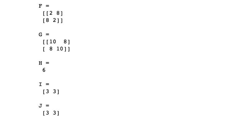

This is just a basic coverage of a few of the things you could do with matrices. In the next part of this article we will see how to do complex operations and use them in computing activations in a neural network.

AI Graduate aims to organize and build a community for AI that not only is open source but also looks at the ethical and political aspects of it. More such simplified AI concepts will follow. If you liked this or have some feedback or follow-up questions please comment below.

Thanks for Reading!